
Graphing!
In our last two Learning Resources, we looked at two fundamental elements of Mathematics, Algebra and Geometry. In this section, we'll look at the marriage of these two ideas, graphing.
A Marriage of Maths and Art
Graphing is visually what our algebraic equations look like. If you're confused by what this means or struggle with drawing correct graphs in school, follow us in this step-by-step guide to the basics of graphing.
The Number Line
First, let's look at something familiar, the number line. On this line are all the numbers we know, 0, 1, 2, −1, π.
We can use our operators (+, −, ×, ÷) to move along this line.
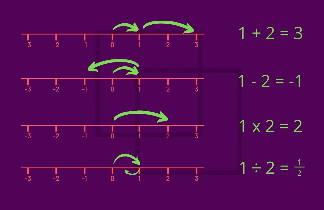
Check out our Algebra Resource for how to use these operators on variables.
The Number Plane – The Coordinate System
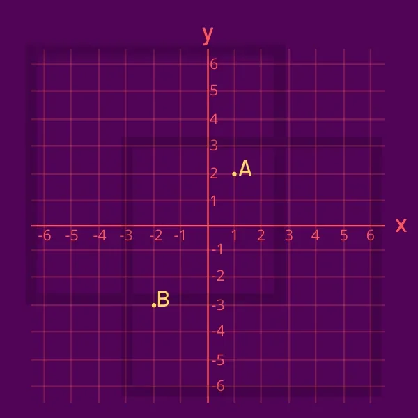
Now that we've covered the number line, let's add another one, this time vertical instead of horizontal so that we get a number plane.
We'll call the horizontal axis the x-axis, and the vertical axis the y-axis.
Just like how we have numbers on a number line, we have coordinates on a number plane.
We write these coordinates as (x,y) where x is the number left or right on the x-axis and y is the number up or down on the y-axis.
Here we see the point A is 1 unit right and 2 units up, so A = (1,2). Similarly, B is 2 units left and 3 units down, so B = (−2,−3).
The point where the axes meet is the Origin, which is at (0,0).
The Four Quadrants
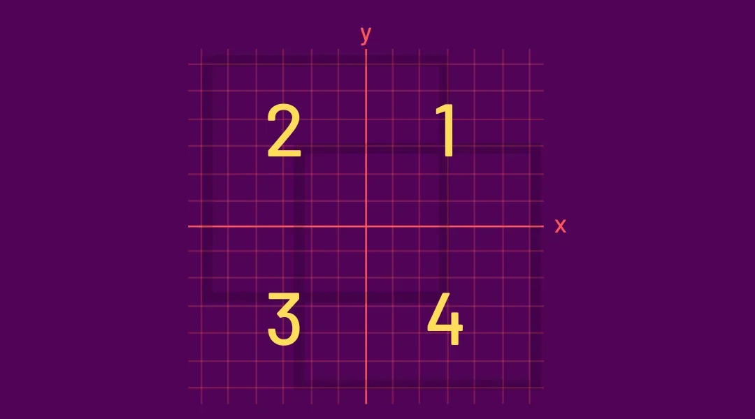
If we look at our number plane, we can see that it's split up into four sections, which we call quadrants.
1st Quadrant
The first quadrant is where both x and y are positive.
2nd Quadrant
The second quadrant is where x is negative and y is positive.
3rd Quadrant
The third quadrant is where both x and y are negative.
4th Quadrant
The fourth quadrant is where x is positive and y is negative.
Graphing Equations – Constructing a Table of Values
In this section, we'll look at drawing some basic algebraic equations.
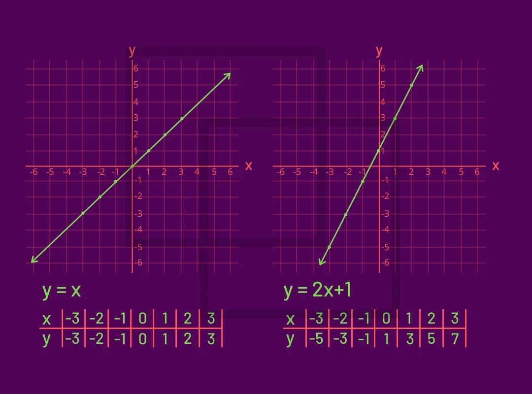
We'll start with an easy example, y = x.
The first thing to do with these equations is to draw up a table of values. We start with some basic values of x (−2, −1, 0, 1, 2, 3) and see what values we get for y.
Each column gives us a pair of coordinates, i.e. (−2,−2), (−1,−1) etc. So, all that's left to do is join the dots and we get a line.
Let's try a trickier example, y = 2x + 1.
"I'll do Algebra, I'll do Trig, but Graphing is where I draw the line."
Distance and Midpoint
In this section we'll be looking at some more geometric features of graphing, such as distance and midpoint.
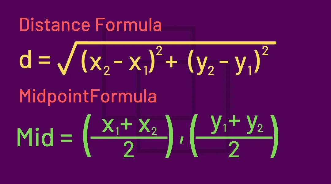
1. Distance
To find the distance between two points, (x1, y1) and (x2, y2), we use the distance formula. Although this may seem complicated, it is derived from Pythagoras' Theorem (which we looked at in the Geometry Resource).
2. Midpoint
To find the midpoint between two points, (x1, y1) and (x2, y2), we use the midpoint formula, which simply takes the average of two points.
Gradient
In the next few sections, we'll look at two key concepts to graphing, gradient and intercepts.
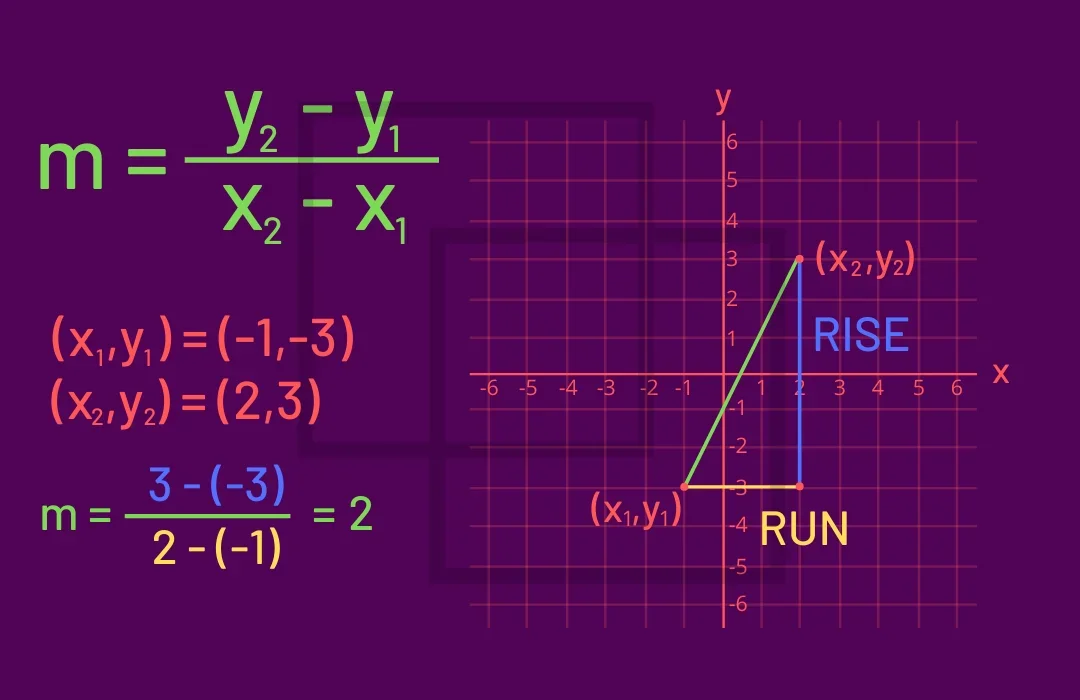
Firstly, gradient is the slope of a graph and you'll commonly hear it as RISE/RUN, where RISE is the change in y and RUN is the change in x.
To find the gradient (which we call m), we need to know two points on the graph (x1,y1), and (x2,y2).
The formula to find the gradient is shown below.
For example, if we have two points, (−1,−3) and (2,3), we can calculate the gradient.
Intercepts
Intercepts are the second important concept to graphing.
These are the points where our line meets the x- and y-axes.
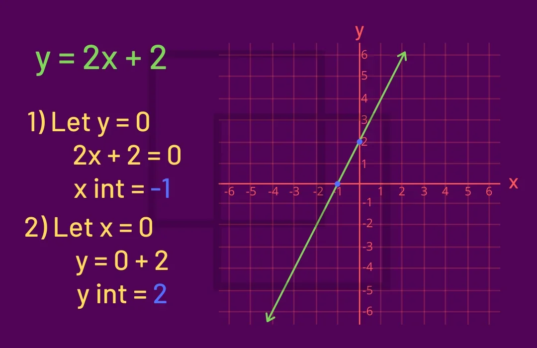
To find the intercepts of a graph, we let the other variable equal 0.
So if we want to find the x-intercept (where the graph meets the x-axis), we let our y = 0. Similarly, to find the y-intercept (where the graph meets the y-axis), we let x = 0.
For example, we have a graph y = 2x + 2.
Gradient-Intercept Formula
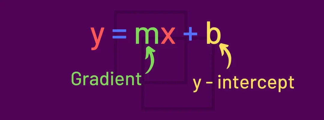
Now that we know what gradient and intercepts are, and how to calculate them, we can make a general formula to describe every straight line.
This formula is called the gradient-intercept because all we need to know is the gradient, and the y-intercept, and we know our straight line.
For example, a line with a gradient of 2 which intersects the y axis at y = 2 has equation y = 2x + 2.
Point-Gradient Formula
However, you may find it is sometimes difficult to find the Gradient-Intercept form of a line, especially when you don't know the y-intercept!
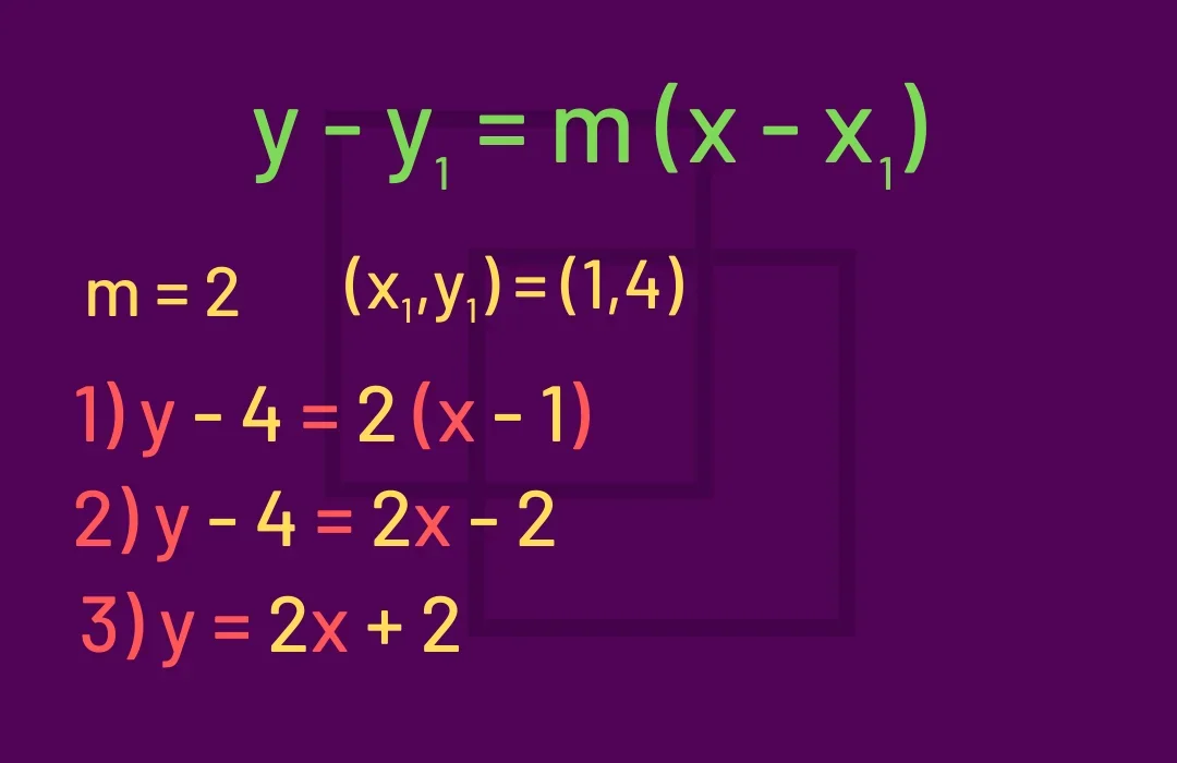
But don't worry, we have another tool in our graphing toolbox, and that's the Point-Gradient formula.
For this formula, we need to only know a point on the line (x1,y1) and the gradient (m). Then we simply substitute into the formula.
For example, if we have a line which passes through (1,4) with gradient 2, we find a unique equation of a line.
Graphing the Parabola
Up until now, we've been looking at graphs that are straight lines. However, straight lines only make up a small number of graphs.
In this section, we'll be tackling the famous parabola.
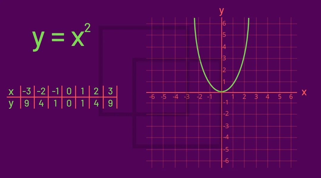
In the Algebra Learning Resource, we learnt about quadratics. Just as straight lines are defined by the equation y = mx + b, parabolas are defined by quadratics, y = ax2 + bx + c.
Let's look at the standard parabola, y = x2. Our first step should always be to construct a table of values.
Confused by quadratics? Don't stress, check out our Algebra Resource page for more information!
Variations in the Parabola
Just as there are variations in straight lines, there are also variations in parabolas.
We define the gradient of a parabola as the coefficient of the x2 term.
Changing the Slope
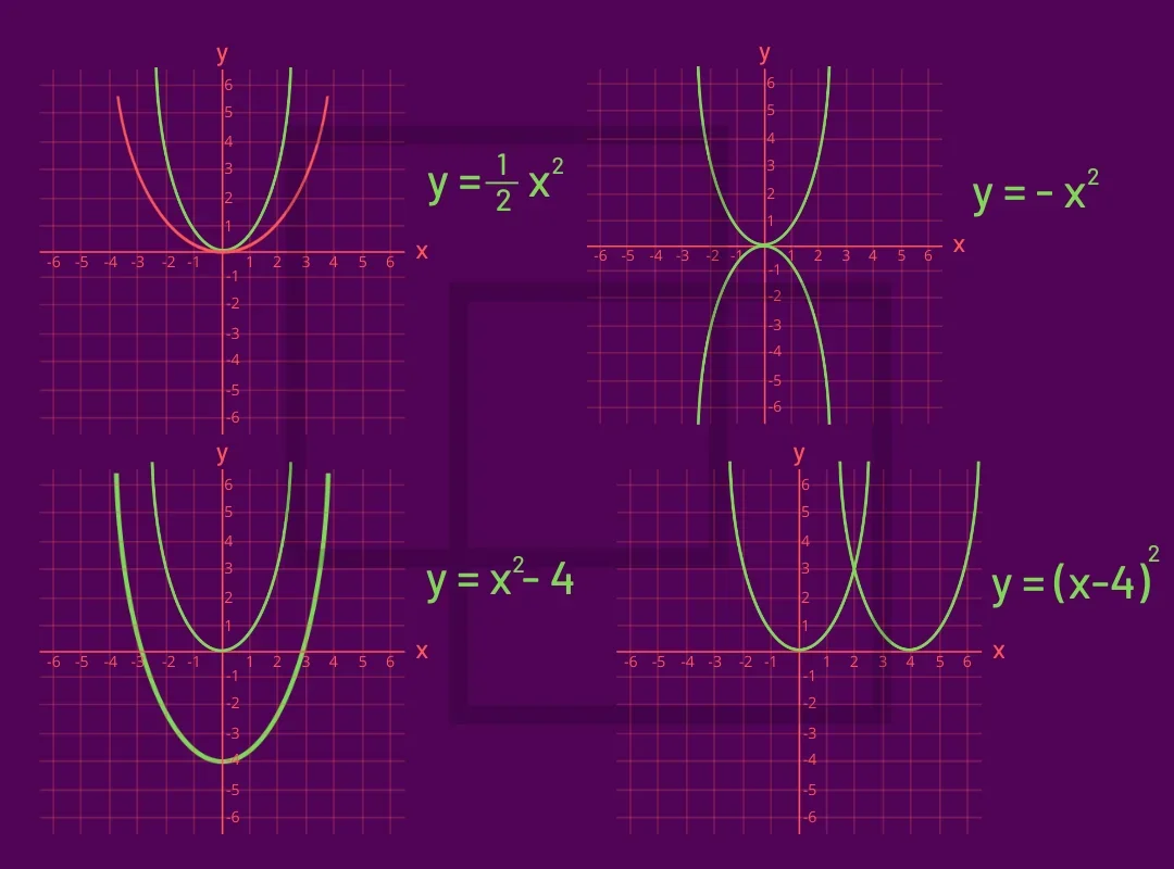
We can make our parabolas steeper or flatter by changing the gradient.
A larger gradient corresponds to a steeper parabola, whereas a smaller gradient corresponds to a flatter parabola.
The Negative
In the case of a negative gradient, the parabola is flipped over the x-axis.
Vertical Shift
We can shift the parabola up (+) or down (−) by a units:
y = x2 ± a
Horizontal Shift
We can shift the parabola left (+) or right (−) by a units:
y = (x ± a)2
When in doubt with how a quadratic is shifted or changed, just plug in a table of values!
Still Struggling with Graphing?
Sometimes the internet just isn't enough and you really do need a mentor to guide you in person.
Smart Space offers in person lessons with engaging tutors. Maybe we can help you. Take a look at our Maths courses or book a free trial below.